Why Are “Asymmetric” Power Laws Necessary for Reasoning?
Published:
Uniform sampling sounds obviously right for long-tail learning: rare skills need more examples. But for compositional reasoning, that intuition can be exactly wrong. Uniform data fails due to worse landscape, but power-law data breaks the symmetry and creates a slope.
Links: paper, PDF, and Eric Michaud’s quanta essay.
The question
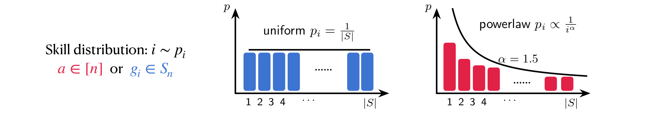
If language is made of many small pieces of knowledge and computation, should we make their training frequencies uniform?
The tempting answer is yes. A model has to learn common things, like basic syntax and frequent relations, but also rare things: a specific person’s advisor, an uncommon arithmetic operation, a niche entity, a long-tail relation, or a small algorithmic trick. If rare skills are the problem, flattening the distribution seems like the obvious fix.
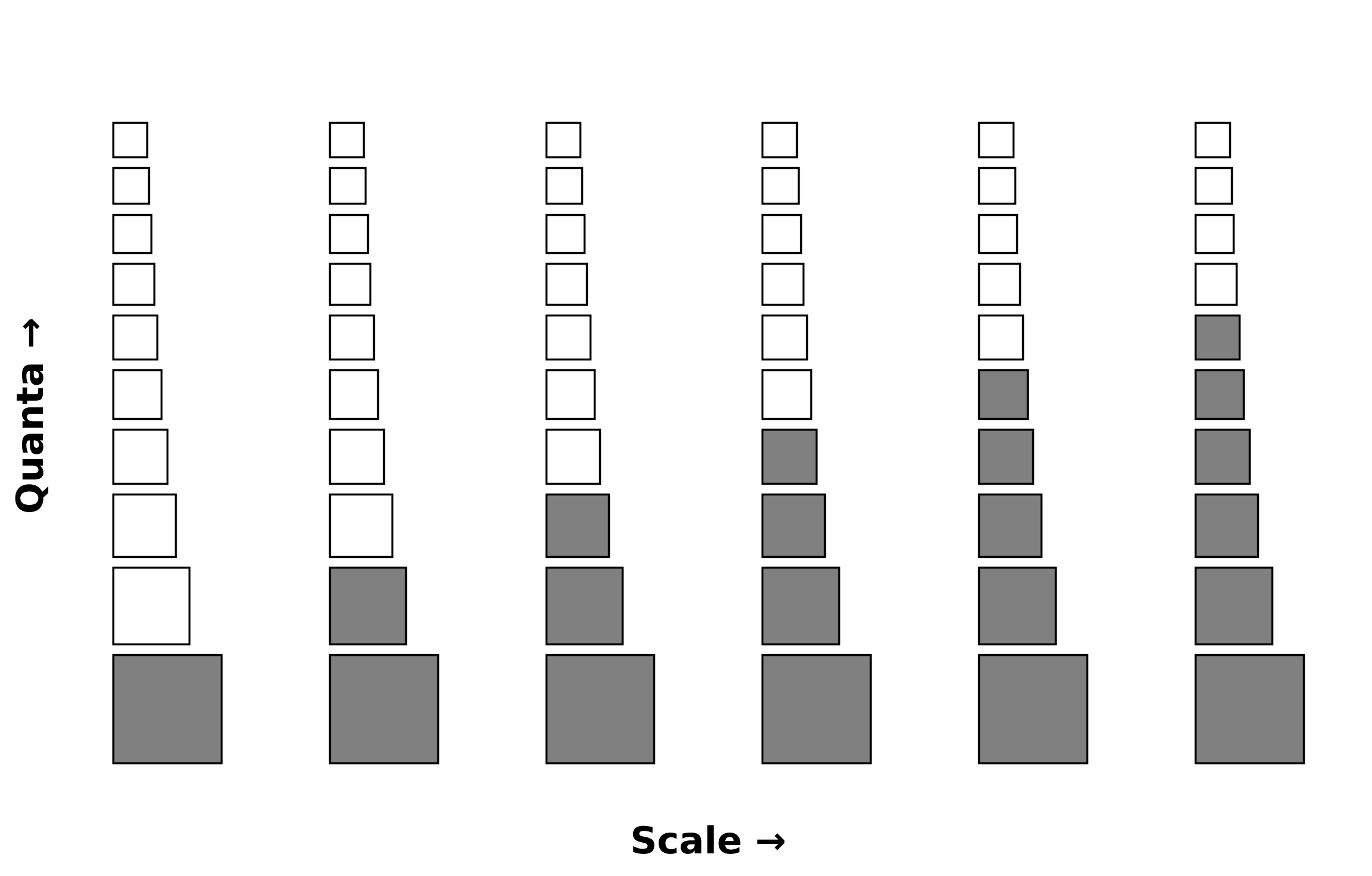
Michaud’s quanta view is a useful way to motivate the setup: pretraining may involve many discrete modules, some retrieving knowledge and some implementing small algorithms, with very different use frequencies. One of the assumptions is:
The "use frequencies" of the quanta naturally follow a power law.
Eric Michaud, On neural scaling and the quanta hypothesis
Our paper, The Power of Power Law: Asymmetry Enables Compositional Reasoning, then asks a more optimization-focused question: what happens when the model does not merely recall one quantum, skill, or fact, but must compose several of them?
But if the task is multi-hop? This is where the long-tail intuition starts to wobble. A multi-hop example is not just a rare item; it is a product of several items that all have to line up.
The answer is not just “the head helps the tail.” The sharper point is geometric: uniform sampling makes the compositional task too symmetric. Near initialization, gradient descent sees a flat, isotropic landscape. Power-law sampling breaks that symmetry, tilts the landscape, and gives SGD a direction before the model has learned anything useful.
Why uniform looks right
Start with memorization. If a relation or entity appears rarely, the model needs more direct exposure to it. In this setting, uniform sampling is the natural fix because the bottleneck is coverage.
Fact: Anya -- father --> Loid
Question: Who is the father of Anya?
Answer: Loid
That intuition shows up cleanly in a one-hop QA experiment. We randomly rank relations, train under either a uniform or power-law distribution, and evaluate exact match. Uniform wins the early race.
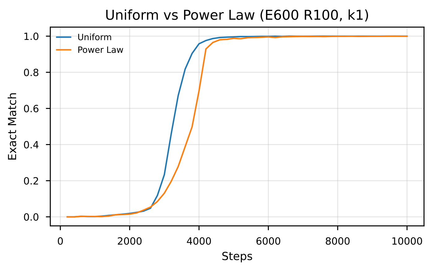
If the task were only to store isolated facts, “use a power law” would be a strange recommendation. The head is already frequent; the tail needs data. Flattening the distribution gives every skill a fairer chance.
Now change only the task. Instead of asking for one relation, ask for a chain. The model must apply one relation, keep the intermediate entity around, and then apply another relation.
Fact 1: Alice -- advisor --> Bob
Fact 2: Bob -- institution --> Princeton
Question: What is the institution of Alice's advisor?
Answer: Princeton
This is a small change in surface form, but a large change in the learning problem. In one-hop QA, each relation can be learned almost independently: see enough examples of the relation, store the mapping, retrieve it later. In two-hop QA, the model has to retrieve the first fact, use its answer as the input to the second fact, and only then produce the final answer.
This makes the uniform intuition even more tempting. If a chain uses $k$ skills with frequencies roughly $p_1,\ldots,p_k$, the full combination is much rarer than any one skill alone. From a pure coverage view, power law should look especially bad here: it undersamples the tail, and rare chains involve rare pieces.
So the naive prediction is: uniform should help more for multi-hop reasoning than for memorization.
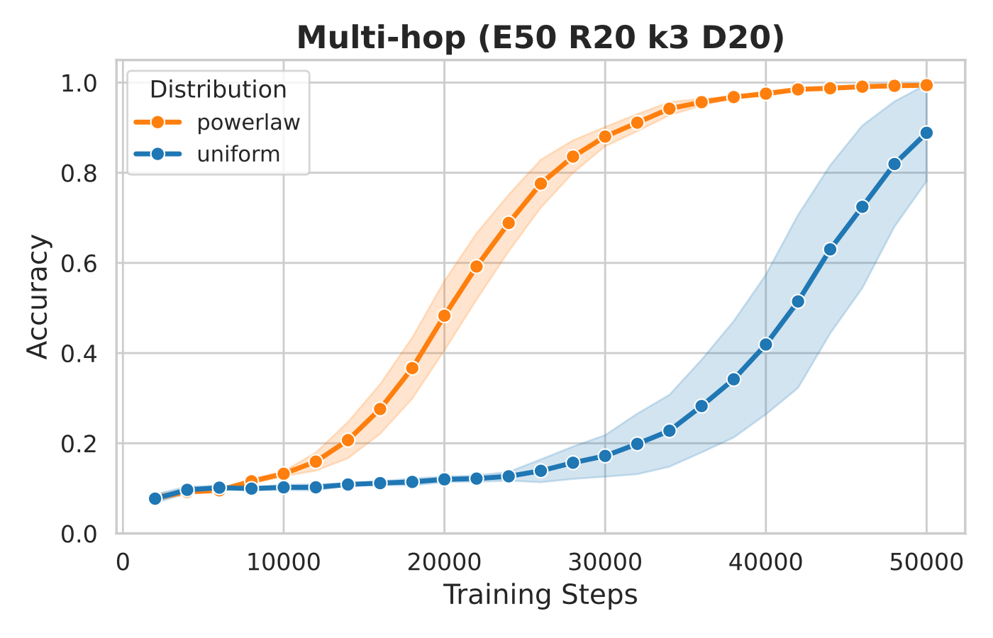
But the experiment goes the other way.
The question is no longer “is uniform good or bad?” The question is: what changes when a model has to compose skills rather than recall them one at a time?
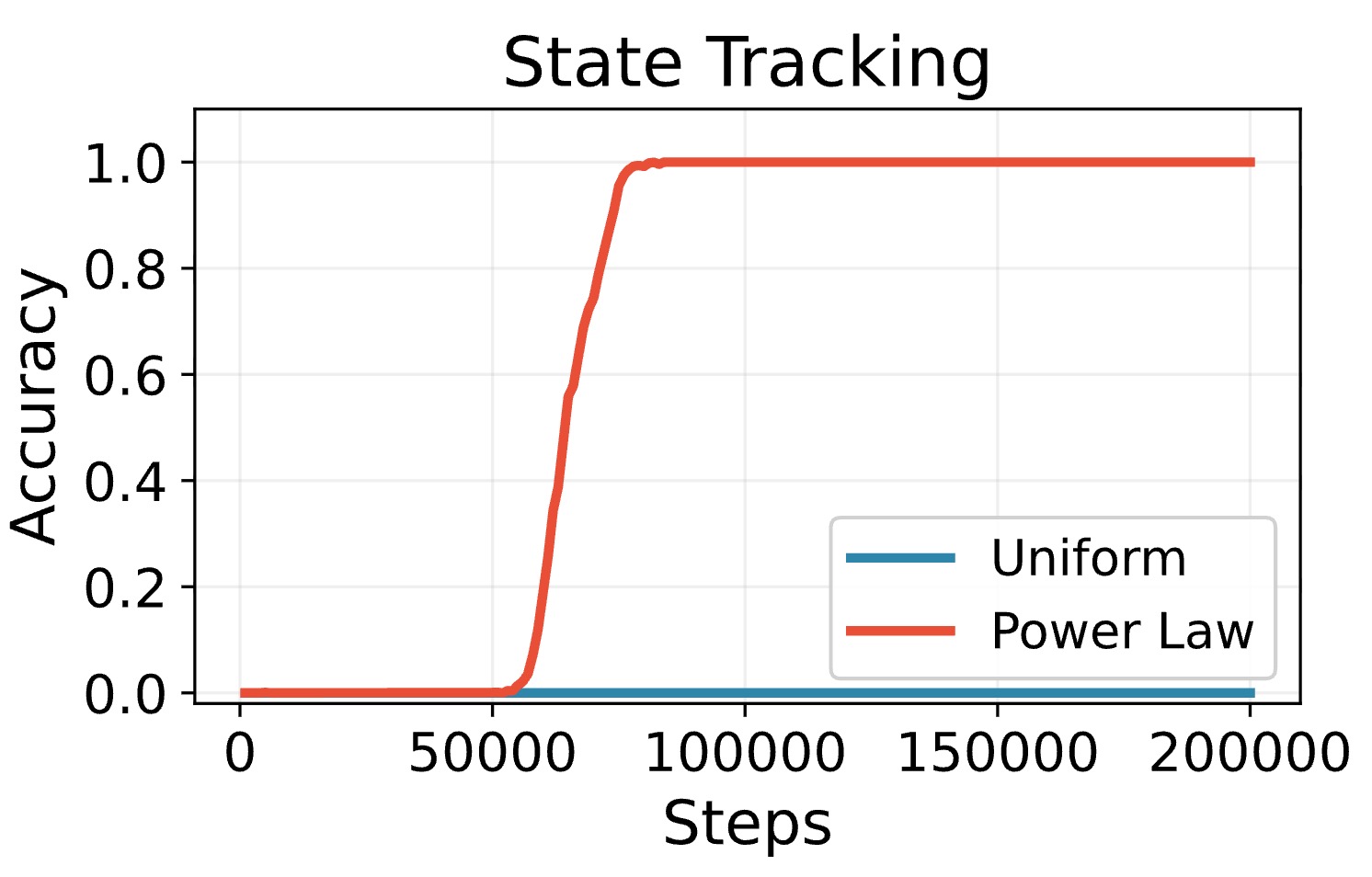
A clean state-tracking testbed
A useful abstraction is $k$-fold composition. Think of each relation, operation, or state update as a function. A reasoning example asks the model to apply several functions in order before answering.
State tracking is a clean synthetic testbed for implicit composition, related to Allen-Zhu’s DePO/canon-layer setup, Merrill and Sabharwal’s transformer limits work (parallelism, chain of thought), and our curriculum study. The model observes updates and must output the final state, so knowing one update rule is not enough; it has to carry state through several steps.
In our experiment, the difference is stark: uniform training stays near zero accuracy, while power-law training escapes and solves the task. That is the first hint that the distribution is changing optimization geometry, not just coverage.
Starting from this synthetic task, we confirmed the same qualitative finding: changing the training distribution can turn an apparently unlearnable implicit composition task into a learnable one. But transformers are still hard to analyze directly: attention, layers, finite samples, and representation learning are all mixed together. To understand the mechanism, we now strip the task down to the smallest model that still contains composition.
Why uniform creates a symmetric hard instance
To isolate the landscape mechanism, use the smallest compositional world possible.
There are $d$ skills. Skill $i$ has a hidden sign $w_i^\star$, equal to either $-1$ or $+1$. A training example samples $k$ skills from a distribution $p$, and the label is the product of their hidden signs:
\[y=\prod_{t=1}^k w^\star_{I_t}.\]The model stores one parameter $w_i$ per skill and predicts the same kind of product:
\[f_w(X)=\prod_{t=1}^k w_{I_t}.\]This model is not meant to be realistic. Its job is to separate two effects:
- For $k=1$, learning is local. Each example updates one skill.
- For $k>1$, learning is global. A skill is useful only when it agrees with the other skills in the product.
The mechanism. The important quantity is the weighted alignment
\[A(w)=\sum_{i=1}^d p_i w_iw_i^\star.\]Think of $A(w)$ as the statistic that tilts the landscape toward the hidden target. If $A(w)$ is large, the model has a rough global sense of the target. If $A(w)$ is tiny, the landscape is nearly flat in the useful compositional direction.
To see where this comes from, train with population squared loss
\[\mathcal L(w)=\frac12\mathbb E_X\left[\left(f_w(X)-f_{w^\star}(X)\right)^2\right].\]Also define the weighted norm
\[B(w)=\sum_{i=1}^d p_iw_i^2.\]Because the sampled skills are independent,
\[\mathbb E[f_w(X)^2]=B(w)^k,\qquad \mathbb E[f_w(X)f_{w^\star}(X)]=A(w)^k.\]So the loss becomes
\[\mathcal L(w)=\frac12\left(B(w)^k-2A(w)^k+1\right).\]The first term is the model’s own scale. The second term is agreement with the hidden target. The third term is constant.
Differentiating gives
\[\nabla \mathcal L(w) =kD\left(B(w)^{k-1}w-A(w)^{k-1}w^\star\right), \qquad D=\mathrm{diag}(p_1,\ldots,p_d).\]The useful part of the negative gradient for skill $i$ therefore scales like
\[p_iA(w)^{k-1}.\]This is the landscape mechanism in one line.
The factor $p_i$ is local coverage: how often skill $i$ appears. Uniform sampling helps this term for tail skills. The factor $A(w)^{k-1}$ is the initial slope in the compositional direction. Uniform sampling can make this slope vanish with dimension by making the problem too symmetric.
| Task | What must be large? | What uniform helps | What uniform can hurt |
|---|---|---|---|
| One-hop memorization | Local exposure $p_i$ | Tail coverage | Usually nothing essential |
| $k$-hop composition | Exposure and landscape slope $A(w)^{k-1}$ | Tail coverage | The initial descent direction |
Table 1: Memorization is mostly a coverage problem. Composition is coverage plus a non-flat landscape.
Why symmetry is the problem
Symmetry hides the signal. At random initialization, the model has tiny accidental correlations with the target. The question is whether the training distribution amplifies those correlations into a useful slope or averages them away.
If $w_i(0)\sim \mathcal N(0,r^2)$, then
\[\mathrm{Var}(A(w_0))=r^2\sum_{i=1}^d p_i^2.\]Under uniform sampling, every skill has probability $1/d$, so $\sum_i p_i^2=1/d$. The alignment is an average over all $d$ random coordinates, and its typical size is about
\[\lvert A(w_0)\rvert\approx \frac{r}{\sqrt d}.\]Composition raises this alignment to the power $k-1$. So the useful compositional signal behaves like
\[\left(\frac{r}{\sqrt d}\right)^{k-1}.\]This is the hidden cost of fairness. Uniform sampling gives every skill equal coverage, but near initialization it also washes out the asymmetry gradient descent needs to escape the flat region.
Under a power law, the head skills carry constant-scale probability mass. For $p_i\propto i^{-\alpha}$ with $\alpha>1$, the quantity $\sum_i p_i^2$ no longer shrinks like $1/d$; in the large-$d$ limit it behaves like a constant such as $\zeta(2\alpha)/\zeta(\alpha)^2$. The same random initialization now has
\[\lvert A(w_0)\rvert\approx \Theta(r).\]The tail is still rare. But the head is frequent enough to break the symmetry.
| Sampling rule | Initial alignment | What gradient descent sees |
|---|---|---|
| Uniform | $r/\sqrt d$ | nearly flat composition landscape |
| Power law | $\Theta(r)$ | visible descent direction |
Table 2: Power law helps by making the first descent direction visible, not by making rare skills common.
The formal results in the paper sharpen this picture. Under uniform inputs, a correlational statistical-query lower bound gives a $d^{\Omega(k)}$-type obstruction for gradient-like learning. This is the theorem-level version of the flat-landscape story: the learner cannot cheaply find a correlated direction. Under a Zipf distribution with $\alpha>1$, minibatch gradient descent learns the minimalist composition task with about $\widetilde O(d^{2\alpha})$ samples, up to theorem conditions on step size, batch size, and accuracy.
In other words, the first miracle is not head-to-tail transfer. It is escape.
Uniform removes imbalance. Composition sometimes needs imbalance to create a slope.
What happens inside the transformer?
The toy model makes two concrete predictions for state tracking. First, near initialization, uniform training should look flatter because the compositional direction is hidden by symmetry. Second, after escape, learned head skills should increase the gradient signal for the rest of the skills.
Stage I: escaping the flat region. We visualize the loss over the top two PCA directions of checkpoint trajectories. Under uniform training, the initialization region is nearly flat in this subspace. Under power-law training, the trajectory sees a clearer descent direction.
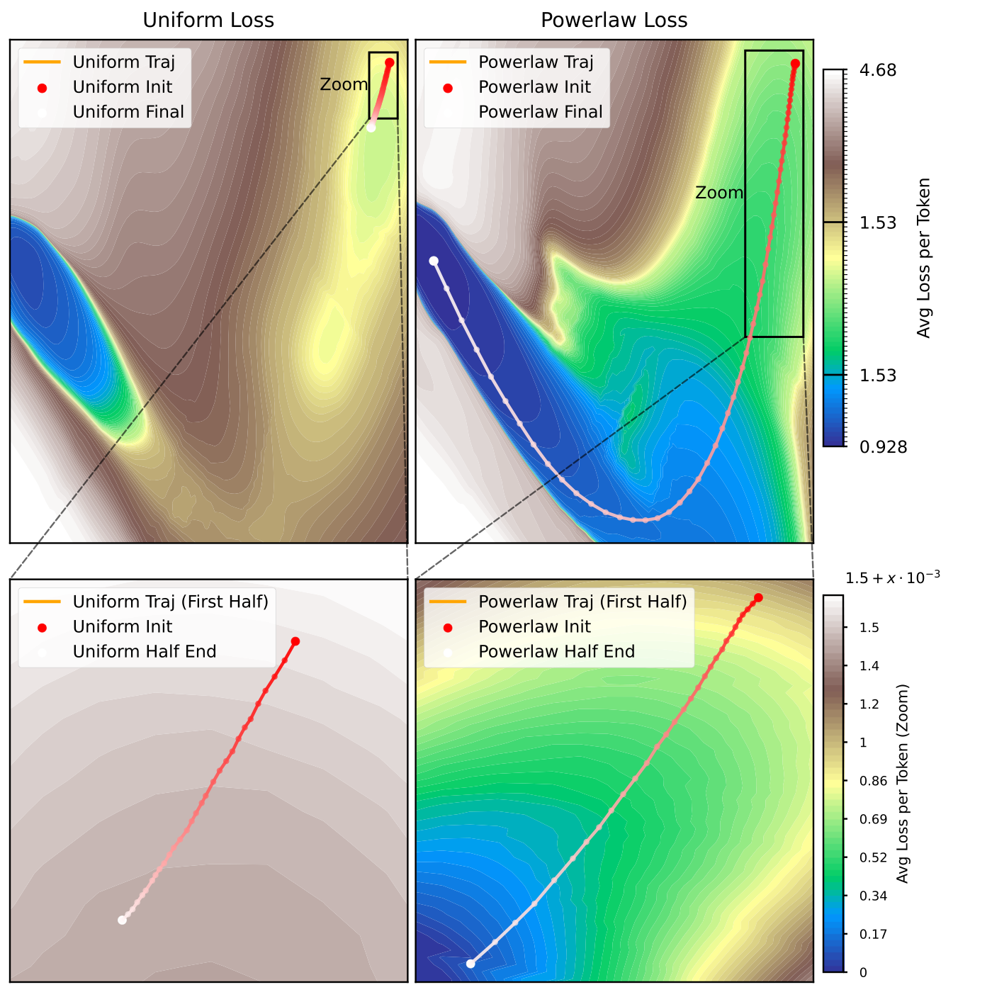
This is the paper’s main mechanism in picture form. The distribution does not merely change which examples are sampled. It changes the shape of the loss landscape near initialization.
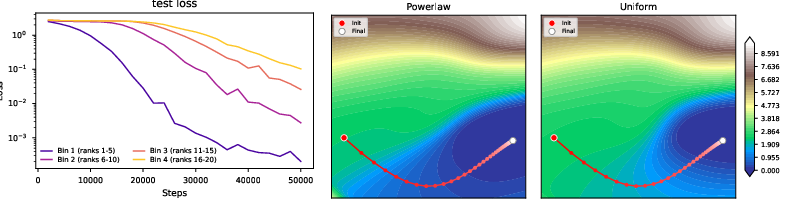
Stage II: the head becomes a handle for the tail
Head first, tail later. Once the model has escaped the flat region, the head plays a second role. Frequent skills learn first. As they align with the target, they increase $A(w)$. That larger alignment then strengthens the useful gradient for every skill, including rare ones.
To check this learning order in the transformer, we group the hidden permutations by rank and track loss, accuracy, and gradient norm. The head group learns first. As it aligns, the gradient norm for later groups grows, and learning moves from head to tail.
So the power law creates a staged learning order: first it breaks the flat symmetric landscape, then learned head skills amplify the signal for rarer skills, and finally the ordinary long-tail problem returns because tail skills are still sampled rarely. These plots are not a theorem for transformers, but they are a mechanistic sanity check: the same signatures predicted by the toy model appear in a real transformer training run.
This is why the result is not “skew is always good.” It is a tradeoff. Too little asymmetry gives no slope. Too much asymmetry starves the tail. The advantage comes from a learning order: escape first, head first, tail later.
Back to reasoning tasks
Why these two tasks? State tracking is useful because it isolates the mechanism, but it is still a laboratory task. We also want to know whether the same signature appears in more language-like reasoning tasks. That is why the paper uses two additional settings.
Multi-hop QA tests relation composition in natural-language form. We generate a synthetic knowledge graph with facts of the form
\[e_i \xrightarrow{r} e_j,\]and ask questions by chaining relations:
\[e_0 \xrightarrow{r_1} e_1 \xrightarrow{r_2} e_2 \cdots \xrightarrow{r_k} e_k.\]Each relation is an atomic skill, but the answer requires several of them in order. The model cannot solve the task by memorizing one edge.
This is close in spirit to work on knowledge manipulation and implicit multi-hop reasoning in language models: the question is whether the model can perform the intermediate hops internally, without being handed the chain of thought.
Facts: Alice's advisor is Bob. Bob's institution is Princeton.
Question: What is the institution of Alice's advisor?
Computation: Alice -> Bob -> Princeton
Facts: Start with 4. Add 3. Then double it.
Question: What number do we get?
Computation: 4 -> 7 -> 14
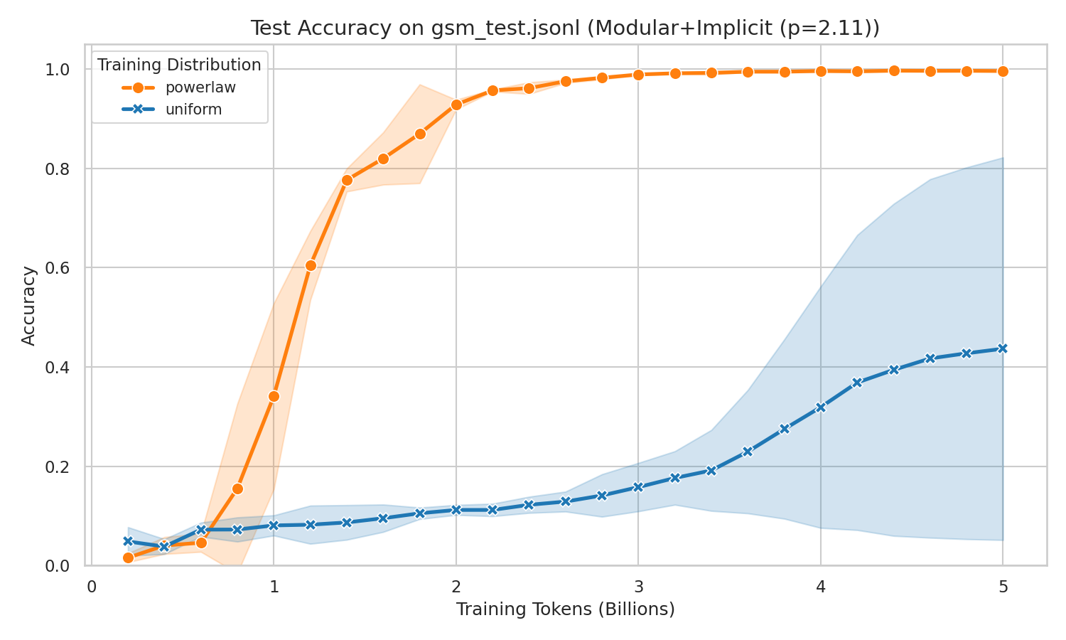
GSM-style arithmetic is a complementary check. It is not about graph relations between entities; it is about composing arithmetic operations through a dependency graph. If power law only helped because of some artifact of relation chaining, this task would be a weaker place to see it. But the same pattern appears.
An intuition
Uniform sampling is like a perfectly balanced table. It is fair, but level: gradient descent has no obvious way to roll.
Power-law sampling puts weight on one side. That looks unfair if all you care about is coverage, but now the table has a tilt. Gradient descent can start moving; after that, learned head skills can help pull the tail along.
In the toy model, that tilt is the alignment $A(w)$. The strength of the initial descent direction is controlled by that alignment.
What this suggests in practice
The practical lesson is not “make all training data more skewed.” It is narrower:
- Evaluate memorization and composition separately. A distribution that improves one-hop recall can hurt implicit multi-hop learning.
- Do not treat repeated head examples as automatically wasted. In a compositional task, frequent skills can change the loss geometry.
- Tune the exponent. Larger $\alpha$ can accelerate head learning, but too much skew slows the final tail stage.
- Ask not only “does the tail get enough examples?”, but also “does this distribution create a slope near initialization?”
What this does not show
- The result does not say power law is always better. In one-hop memorization, uniform sampling learns faster.
- The theorem is for a minimalist $k$-multiplicative composition model, not a full transformer theory.
- The positive theorem assumes a Zipf distribution with $\alpha>1$, constant even $k$, Gaussian initialization, and a learner matched to the compositional structure.
- The lower bound is for uniform or symmetric input distributions and correlational statistical-query learners, which include gradient-like methods but not every possible algorithm.
- The experiments are synthetic: state tracking, synthetic multi-hop QA, and synthetic GSM-style arithmetic.
- Other asymmetric distributions might also help. The paper treats power law as a natural, fine-grained source of asymmetry, not the only possible one.
The surprising lesson is that fairness in the data distribution can create symmetry in the loss landscape, and symmetry can be deadly for composition. Power law helps not because the tail becomes common, but because the head breaks the symmetry first. For reasoning, the first problem is not always seeing every skill. Sometimes it is finding any slope at all.
The thing to remember is simple: uniform fixes exposure. Power law fixes the landscape.
References
- Zixuan Wang, Xingyu Dang, Jason D. Lee, and Kaifeng Lyu. The Power of Power Law: Asymmetry Enables Compositional Reasoning. arXiv, 2026.
- Eric J. Michaud. On neural scaling and the quanta hypothesis. 2026.
- Eric J. Michaud, Ziming Liu, Uzay Girit, and Max Tegmark. The Quantization Model of Neural Scaling. NeurIPS, 2023.
- Zeyuan Allen-Zhu. Physics of Language Models: Part 4.1, Architecture Design and the Magic of Canon Layers. SSRN, 2025.
- Zeyuan Allen-Zhu and Yuanzhi Li. Physics of Language Models: Part 3.2, Knowledge Manipulation. arXiv, 2023.
- William Merrill and Ashish Sabharwal. The Parallelism Tradeoff: Limitations of Log-Precision Transformers. TACL, 2023.
- William Merrill and Ashish Sabharwal. The Expressive Power of Transformers with Chain of Thought. arXiv, 2023.
- Zixuan Wang, Eshaan Nichani, Alberto Bietti, Alex Damian, Daniel Hsu, Jason D. Lee, and Denny Wu. Learning Compositional Functions with Transformers from Easy-to-Hard Data. arXiv, 2025.
- Nouha Dziri et al. Faith and Fate: Limits of Transformers on Compositionality. arXiv, 2023.
- Yuekun Yao, Yupei Du, Dawei Zhu, Michael Hahn, and Alexander Koller. Language Models Can Learn Implicit Multi-Hop Reasoning, but Only if They Have Lots of Training Data. arXiv, 2025.
- Sanjeev Arora and Anirudh Goyal. A Theory for Emergence of Complex Skills in Language Models. arXiv, 2023.
- Michael Kearns. Efficient noise-tolerant learning from statistical queries. Journal of the ACM, 1998.
- Yoshua Bengio, Jerome Louradour, Ronan Collobert, and Jason Weston. Curriculum Learning. ICML, 2009.
- Aaron Clauset, Cosma Rohilla Shalizi, and M. E. J. Newman. Power-law distributions in empirical data. SIAM Review, 2009.